Low‑Frequency Dipole Noise Mechanisms in Stalled Aerofoil

Date/revision:

20 August 2026

southmeta_1 Authors: Douglas W. Carter ^✉ Bharathram Ganapathisubramani ^✉

Affiliation : Department of Aeronautics and Astronautics, University of Southampton, United Kingdom.
✉ dcarter10@illinoistech.edu, G.Bharath@soton.ac.uk

Introduction

Airflow around objects, from aircraft wings to road vehicles, generates forces and noise that are governed by the distribution of pressure in the flow. While pressure is a fundamental quantity in aerodynamics, it is difficult to measure directly across an entire flow field.

Modern optical techniques such as Particle Image Velocimetry allow the velocity of the fluid to be captured in a non intrusive manner, providing a detailed view of complex flow behaviour. Using these velocity measurements, the pressure field can be reconstructed by applying the governing equations of fluid motion^[1,2,3]. In incompressible flows, this is achieved by solving a pressure Poisson equation derived from the Navier Stokes equations, linking pressure to the temporal and spatial variations of velocity. This approach enables the estimation of instantaneous and spatially resolved pressure fields that are otherwise difficult to obtain experimentally.

This dataset focuses on the flow over a NACA 0012 aerofoil under stalled conditions, where pressure fields are reconstructed from time resolved velocity measurements and compared with numerical simulations. The data provide insight into unsteady flow structures and their role in aerodynamic noise generation, offering a valuable resource for validation, modelling, and the development of quieter and more efficient aerodynamic systems.All results from these measurements can be found in Carter and Ganapathisubramani^[4], which offers a detailed description of the test conditions and wind tunnel setup.

Model Geometry

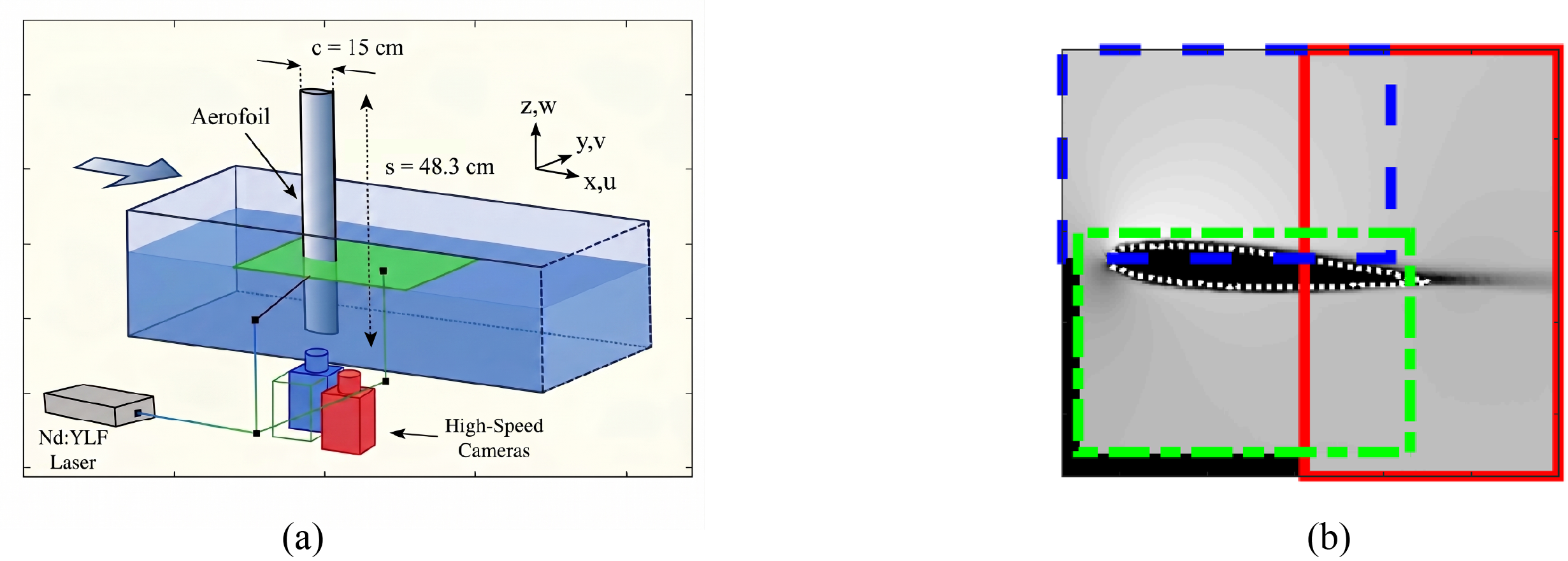
The model used in this study is a NACA 0012 aerofoil, a symmetric profile widely used as a reference geometry in aerodynamic research. The aerofoil has a chord length of 0.15 m and is mounted vertically within the test section of a water flume. The total span of the model is 0.70 m, of which approximately 0.483 m is submerged in the flow, ensuring a sufficiently large aspect ratio within the measurement region.

The aerofoil is positioned at the centre of the test section, aligned such that the measurements are performed in the streamwise and surface normal plane passing through the mid span. The flow is directed along the chordwise direction, and the measurement plane captures the suction side, pressure side, and trailing edge regions of the aerofoil.

The angle of attack of the aerofoil is precisely controlled using a mounting system, allowing systematic variation of the flow conditions. In this dataset, measurements are conducted at 13°, and 15° angle of attack, representing transitional stall, and deep stall regimes respectively. These configurations enable the investigation of flow separation, shear layer development, and their influence on the resulting pressure field and aerodynamic noise.

Figure 1. Distribution of PIV planes used in this study.

Measurement Location and Techniques

The flow field was measured using time resolved Particle Image Velocimetry, providing planar velocity data in the streamwise and surface normal plane of the aerofoil. Measurements were conducted at the mid span location to minimise three dimensional effects and to capture the dominant flow features associated with separation and wake development.

The flow was illuminated using a laser sheet aligned with the measurement plane, and images were captured using three high speed cameras positioned to cover different regions of the field of view. The cameras were arranged to simultaneously record the suction side, pressure side, and trailing edge regions, enabling a complete view of the flow around the aerofoil. Due to the geometry and viewing angles, a small portion near the pressure side surface was not accessible and was masked during processing.

The individual camera fields of view were processed independently to obtain velocity vectors and then combined into a single continuous domain. This stitching process was performed using calibrated reference images and overlapping regions between adjacent camera views. The velocity fields were aligned and blended to ensure continuity across the full measurement domain, allowing for a consistent reconstruction of the flow field used in subsequent pressure estimation and analysis.

Experimental Facility

The experiments were conducted in a recirculating water flume at the University of Southampton, designed for detailed optical flow measurements. The facility features a test section approximately 6.75 m in length, 1.2 m in width, and 0.5 m in depth, providing a large working area for model testing and flow development. The flow is driven in a closed loop system, ensuring steady operating conditions and allowing long duration measurements required for time resolved diagnostics.

The freestream velocity in the facility is set to approximately 0.5 m/s for the present study, corresponding to a chord based Reynolds number of 7.1 × 10⁴. The facility is capable of delivering stable and uniform flow conditions with low background disturbances, making it suitable for resolving unsteady flow features associated with separation and stall. The use of water as the working fluid enables higher spatial resolution in velocity measurements compared to air based facilities at equivalent Reynolds numbers.

The flume is equipped with optical access along the test section, allowing the use of laser based measurement techniques such as Particle Image Velocimetry. A carriage system is used to mount and position the aerofoil, enabling precise control of the angle of attack. The facility also supports synchronised measurements, including force data acquisition and high speed imaging, providing a comprehensive platform for investigating aerodynamic flow physics and associated phenomena.

Flow Conditions

Freestream velocity = 0.5366 m/s
Chord based Reynolds number (Re_c) ≈ 7.1 × 10⁴
Angle of attack(AOA) = 4°, 13°, and 15°
Flow regimes = attached flow, transitional stall, and deep stall
Working fluid = water
Kinematic viscosity (ν) ≈ 1 × 10^-6 m²/s
Measurement duration per case ≈ 26.8 s
Sampling frequency = 1 kHz
Frequency range analysed = low frequency regime (f* ≤ 3)
f* = non-dimensional frequency (f c / U_∞)
Velocity fields temporally filtered to remove high frequency mechanical noise (> 10 Hz)

CAD files

NACA 0012 profile

Available Datasets

AOA	U_∞	U mean	V mean	U variance	V variance
13°	0.5366	U_mean_13AOA.csv	V_mean_13AOA.csv	U_Var_13AOA.csv	V_Var_13AOA.csv
15°	0.5366	U_mean_15AOA.csv	V_mean_15AOA.csv	U_Var_15AOA.csv	V_Var_15AOA.csv

AOA	U_∞	P mean	P variance	P RANS
13°	0.5366	P_mean_13AOA.csv	P_var_13AOA.csv	P_RANS_13AOA.csv
15°	0.5366	P_mean_15AOA.csv	P_var_15AOA.csv	P_RANS_15AOA.csv

Complete Dataset Archive (ZIP)

The complete original dataset is available here for download and contains both raw and mean measurement data. The original dataset was created and archived by the researchers and it may not be organised in a standardised format. The metadata presented here has been extracted and systematically structured from the original dataset to improve its accessibility, and usability.

Sample plots

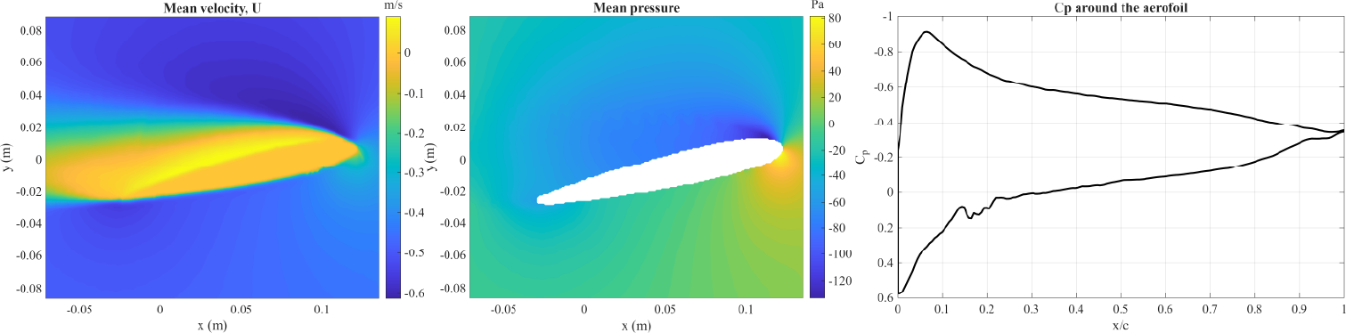
To help you analyze the dataset, a MATLAB script has been provided. This script can be used to automatically create the colour maps of Mean velocity, pressure and coefficient of pressure. The sample plots using the matlab code is given in figure 2.

Figure 2. Sample plots of the mean velocity, pressure, and pressure coefficient distributions around the aerofoil from the dataset at an angle of attack of 13^o.

Open Access

This metadata is provided under the Creative Commons Attribution-NonCommercial 4.0 International License (https://creativecommons.org/licenses/by-nc/4.0/). This license allows for unrestricted use, distribution, and reproduction in any medium, provided that proper credit is given to the original author(s) and the source. Also provide a link to the license, and indicate if any changes were made. Furthermore, this license does not allow the use of this material for commercial purposes.

Acknowledgments

The NWTF acknowledge the support for the metadata work from the EPSRC Network Grant, EP/X011836/1. The original dataset was funded by the Engineering and Physical Sciences Research Council (Ref No: EP/R010900/1) and H2020 Future and Emerging Technologies Project HOMER 769237

Citation

If the user wants to cite the data presented here, then please cite both the NWTF metadata and the corresponding paper^[4].

References

De Kat, R. and Van Oudheusden, B.W., 2012. Instantaneous planar pressure determination from PIV in turbulent flow. Experiments in fluids, 52(5), pp.1089-1106. DOI

Laskari, A., de Kat, R. and Ganapathisubramani, B., 2016. Full-field pressure from snapshot and time-resolved volumetric PIV. Experiments in fluids, 57(3), p.44. DOI

van Gent, P.L., Michaelis, D., van Oudheusden, B.W., Weiss, P.É., de Kat, R., Laskari, A., Jeon, Y.J., David, L., Schanz, D., Huhn, F. and Gesemann, S., 2017. Comparative assessment of pressure field reconstructions from particle image velocimetry measurements and Lagrangian particle tracking. Experiments in Fluids, 58(4), p.33. DOI

Carter, D.W. and Ganapathisubramani, B., 2023. Data-driven determination of low-frequency dipole noise mechanisms in stalled airfoils. Experiments in Fluids, 64(2), p.41. DOI